PID Tuning tool

drbitboy · Oct 8, 2022

P.S. @Peter Nachtwey: I used a Python module a few years ago that takes an XML file as input and generates a schema for it; that comes in useful to validate future inputs. Let me know if you are interested and I will try to figure out what it was.

I don't think you need this, but it also writes Python code suitable for generating XML for that same schema, so you aren't coding the XML strings and structure by hand, but rather constructing an object via simple calls, and that object "knows" how (has a method) to write itself to an XML document. It was pretty slick.

drbitboy · Oct 8, 2022

Peter Nachtwey said:
but it converts the whole file I need only the motion data.

Isn't that a one-liner? E.g.



motion_data = dict(**[(key,all_data[key],)

                      for key in

                      "motion_key0 motion_key1 motion_key2 ...".split()

                     ]

                  )

Even better, put the keys you are interested in into a set and ignore all but those columns when parsing the input CSV (I am pretty sure pandas has summat like that built-in to its read_csv method).

Peter Nachtwey · Oct 8, 2022

drbitboy said:
Isn't that a one-liner? E.g.

motion_data = dict(**[(key,all_data[key],)
for key in
"motion_key0 motion_key1 motion_key2 ...".split()
]
)

Even better, put the keys you are interested in into a set and ignore all but those columns when parsing the input CSV (I am pretty sure pandas has summat like that built-in to its read_csv method).

I am more concerned about how destination unknown's source fudge the formulas for the PID. The formulas seem to work but my formulas work with less over shoot but the trade off is a slower response.

I am suffering from a pinched nerve that is making my left arm go numb after moving my left arm a bit. I can't drive or type with my left arm. I can't drive long enough to go camping. I have been told it will go away after a few months or years. Screw that. I need to make the most of the time I have left.

destination unknown · Oct 10, 2022

Peter Nachtwey said:
The formulas for the controller gains in #116 look reasonable. However, in step 4 they admittedly fudged things. I spent some time trying to do the math without fudging. The document is right. You don't end up with a PID. I failed to have a good/easy solution without fudging.

The authors made a decision to sacrifice purity for simplicity.
Also, the documents technique is a little different from the method used to generate the formulas for row A and B above. It looks like they inverted the plant transfer function and added a low pass filter. Inverting the plant transfer function results in generating the feed forward gains. The document then adds a low pass filter or the response will have a first order response.

I would like to have a copy of the data used to generate the plot in #116

Our motion controller supports using PIs and PIDs but we also go beyond to improve response. As long as the customer doesn't need to deal with the added complexity but only benefits then all is good.

The response shown in the last plot is not that good. There is way too much over shoot. In my last plot the dead time was 10 times longer than the plant time constant.

OT but somewhat related. I have been working on python code to use .json files in addition to .csv files.

Currently I can import a .csv file with the first line being text to describe the columns of time, output, and PV and then as many rows of numbers of time, output and PV.

I am also working on importing accelerometer data acquired from test systems and then using FFTs and IFFTs to filter the data.

For some reason our software group exports motion data in xml or gzipped xml format. Since I do most of my work in python now I need to covert this data to python dictionaries or .json files.

As with all tuning rules there is a trade off.

I didn't save that data as it was an on the fly adaptive tune, the video is here: https://youtu.be/_0bZJYixSdU

The overshoot is pre-tune as the starting PID gains were picked at random, the change in Setpoint shows the tuned response.

MaxK · Oct 26, 2022

destination unknown said:
And the final form of the AutoTuner (SOPDT example):

I will allow myself to express a few thoughts

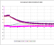
1. Noise and D-term

In my opinion, the CV-noise in your example is unacceptable - it will cause a quick breakdown of the actuator.

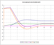
Below I show few graphs with model from your example (2,52 *exp(-4,25*s)/ ((59,80915921*s+1)*(0,460840787*s+1))

- look at the graph “DU model kp=1,9942 ki=0,0329 kd=1,6834” with noise - CV is unacceptably noised
- look at the graph “DU model kp=1,9942 ki=0,0329 kd=0” with noise - CV is quite smooth

As you can see D-term increasing CV-noise

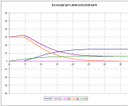
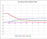
2. Is the D-term useful with your PID-settings?

- look at the graph “DU model kp=1,9942 ki=0,0329 kd=1,6834” without noise
- look at the graph “DU model kp=1,9942 ki=0,0329 kd=0”

PV with kd=0 reaches setpoint faster than with kd=1.6834

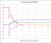
3. Is the D-term useless at all?

- look at the graph “DU model kp=3,36 ki=0,0546 kd=5”
- look at the graph “DU model kp=3,36 ki=0,0546 kd=0”

As you can see it is possible to get system with faster response without overshooting (kd=5). The same system without D-term have overshooting. i.e. in this case D-term is useful.

4. What will be the PID settings for disturbance suppression?

If I'm not mistaken, someone already wrote in this topic that kd is a function of noise parameters, polling frequency (data density) and process dynamics. But not a function of plant parameters.

MaxK · Oct 26, 2022

Peter Nachtwey said:
Velocity and temperature control systems are non-integrating or type 0 systems. Some people call them self regulating.

I do understand difference between integrating and non-integrating systems.

I didn't get how your answer

“Actually, no. Your examples in the past have been for non-integrating systems”

related to my question

“All in all. What was the reason to show me this movie?
Do you think I don't know that 99% for PID-tuning use simplified models?”

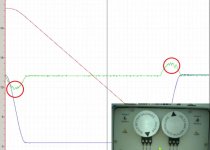
Let's look at the parts of the CO curve in red circles from your video

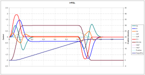
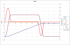
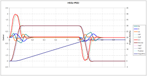
I simulated the system with your plant parameters (600/(s*(2.523763*s+1))) and PID controller settings (please find it in figure “I+FOL”). As you can see, the CO curve is smooth, but in your video the CO curve on the selected fragments is "trembling".

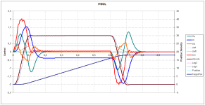
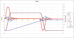
Then I simulated the system with Integrator + 2 order Lag (please find it in figure “I+SOL”). As you can see, the CO curve is "trembling". I.e. the model (600/(s*(2.523763*s+1))) did not take into account all the parameters of the plant that are significant for setting up the PID controller.

Obviously that such CO has an unfavorable effect on the motor.

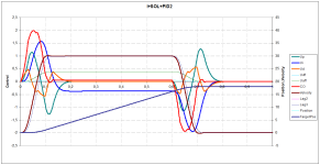
To decrease the "trembling", I applied a second order derivative (please find it in figure “I+SOL+PID2”)

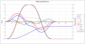
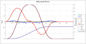
Another way that I have applied to reduce "trembling" is to use a smoother Target position curve (please find it in figure “I+SOL smooth TPcurve”).

MaxK · Oct 26, 2022

Peter Nachtwey said:
I have done many tests comparing different types of ramps. They all have their pluses and minuses like complexity. Even 3rd order ramp problems can be extremely difficult to solve. There is a thread about that a few years ago. Search for the user name cheeco.

I found this thread. But unfortunately the links you shared are now empty. Therefore, I had to independently model the target position curves.

I've attached the motor and target position model file ("motor TP1.xlsx") if somebody interested at. Due to file size limitations, I had to "cut" data. To get the data, just copy line 8 upto 10000.

Peter Nachtwey · Oct 26, 2022

The "trembling" is due to using an actual system with only a 2000 ppr encoder and I was not using an observer to simulate a higher resolution feed back. The controller will multiply this by 4 because it looks for phase changes. The resolution still isn't good enough to calculate very smooth speeds at a millisecond to millisecond time period. The motor is only a 200W motor are there is no velocity loop. The "drive" or amplifier only converts +/- 10 volts to a PWM signal to the small motor. I don't like to use the velocity loops in drives unless it is a simple system.

The derivative gain is critical for stability because the motor and wheel mass rotate freely so if I used only proportional gain, the wheel would oscillate back and forth for a long time because there is little mechanical damping. My motor system was not meant to be easy control. It was meant to be cheap, small, safe, and difficult. Some on this forum have been to our place and have seen our test systems. If you can do the difficult then most will be easy.

Excel, python, Mathcad etc simulations have the benefit of having almost infinite resolution. There should be no problem computing accurate velocities and accelerations.

Your feed forwards are not set correctly. If they were the PID control would only need to correct for small errors. Also, there is no need for a second derivative gain because there are only two poles in the open loop system. One trick we teach people in our class is to plot the integrator's contribution to the total control. It is easy to see where the integrator is winding up or winding down. If the integrator is winding up during the constant velocity phase of the motion then the velocity feed forward is not set right. If the integrator is winding up during acceleration then the acceleration feed forward is not set right. If the feed forwards are set right then the integrator should not vary from 0.

We have controlled some very large systems and some very small ones that move so fast you need a high speed camera to tell what is going on. Big or small, it doesn't really matter except to the power and response of the actuators. We are only shuffling around electrons at almost the speed of light. I have videos. What we do works well.

destination unknown · Oct 26, 2022

MaxK said:
I will allow myself to express a few thoughts

1. Noise and D-term

In my opinion, the CV-noise in your example is unacceptable - it will cause a quick breakdown of the actuator.

Below I show few graphs with model from your example (2,52 *exp(-4,25*s)/ ((59,80915921*s+1)*(0,460840787*s+1))

- look at the graph “DU model kp=1,9942 ki=0,0329 kd=1,6834” with noise - CV is unacceptably noised
- look at the graph “DU model kp=1,9942 ki=0,0329 kd=0” with noise - CV is quite smooth

As you can see D-term increasing CV-noise

2. Is the D-term useful with your PID-settings?

- look at the graph “DU model kp=1,9942 ki=0,0329 kd=1,6834” without noise
- look at the graph “DU model kp=1,9942 ki=0,0329 kd=0”

PV with kd=0 reaches setpoint faster than with kd=1.6834

3. Is the D-term useless at all?

- look at the graph “DU model kp=3,36 ki=0,0546 kd=5”
- look at the graph “DU model kp=3,36 ki=0,0546 kd=0”

As you can see it is possible to get system with faster response without overshooting (kd=5). The same system without D-term have overshooting. i.e. in this case D-term is useful.

4. What will be the PID settings for disturbance suppression?

If I'm not mistaken, someone already wrote in this topic that kd is a function of noise parameters, polling frequency (data density) and process dynamics. But not a function of plant parameters.

Yes, noise is the main concern when it comes to the derivative gain.
There is an option for a conservative PID tune (very little Derivative) to account for this, an alternative option is to filter the controller output.

Peter Nachtwey · Oct 26, 2022

destination unknown said:
Yes, noise is the main concern when it comes to the derivative gain.

It isn't really noise in the analog sense. It is quantizing error. Basically a real or analog system is being digitized and the lack of resolution causes what looks like noise.

Other sources are sampling jitter where the inputs are not sampled at exactly even intervals.

There is an option for a conservative PID tune (very little Derivative) to account for this, an alternative option is to filter the controller output.

Yes, but after we do the auto tune we have a model and can use the model to make an observer to estimate more accurate actual position, velocities and accelerations. After all, in reality the motor position doesn't jump by counts.

This video is a little longer because it explains a lot more.

https://deltamotion.com/peter/Videos/AutoTuningModelingObserver.mp4
You can see the observer compensates for the lack of a high resolution encoder.

MaxK · Oct 27, 2022

Peter Nachtwey said:
Your feed forwards are not set correctly. If they were the PID control would only need to correct for small errors.

First of all thank you – I find my stupid mistake. Attached corrected files.

MaxK · Oct 27, 2022

Peter Nachtwey said:
The "trembling" is due to using an actual system with only a 2000 ppr encoder and I was not using an observer to simulate a higher resolution feed back.

I included a digital output in my simulation. As seen in the "I+FOL" figure, this causes a slight "sawtooth" CO curve at 0.12 - 0.6 s. But there no any “wave trembling” at CO peaks.

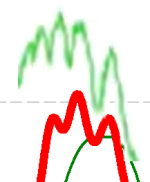
I combined the peak from "I+SOL" with the peak from your video (find it in the picture "CO_d2+videoPeak.png"). The curves seem pretty similar.

Beside, I can't find quantization artifacts in your video (from your post #92 http://www.plctalk.net/qanda/showpost.php?p=923510&postcount=92) in previous experiments (9, 19, 53 sec).

Peter Nachtwey said:
Also, there is no need for a second derivative gain because there are only two poles in the open loop system.

You applied a second-order model, found its coefficients, in response to some impact with some SSE.

As I say in my previous post: The only thing you check this way – how close your models response to plant response “here and now” i.e. at this exact conditions and this exact way.

A real plant is described by a model of a much higher order. To solve some problems, higher orders can be neglected, in other cases it becomes necessary to take higher orders into account.

In this case, after tuning the PID controller, it became noticeable that the second-order model is not enough.

MaxK · Oct 27, 2022

destination unknown said:
Yes, noise is the main concern when it comes to the derivative gain.

Please pay attention to the CO curves even when the signal is not noisy. Are actuators capable of changing their state so quickly?

Peter Nachtwey · Oct 27, 2022

MaxK said:
You applied a second-order model, found its coefficients, in response to some impact with some SSE.

No, I used pole placement.

As I say in my previous post: The only thing you check this way – how close your models response to plant response “here and now” i.e. at this exact conditions and this exact way.

Yes, conditions may vary but not significantly.

A real plant is described by a model of a much higher order. To solve some problems, higher orders can be neglected, in other cases it becomes necessary to take higher orders into account.

No! Poles with shorter time constants can be ignored because they don't make a significant difference to the response. The motor usually has a R/L time constant that I didn't model because it is so short compared to the time constant if the inertia, it can be ignored.

In this case, after tuning the PID controller, it became noticeable that the second-order model is not enough.

You didn't look at the longer video where the control output is very smooth.

I am not sure that the small amplifier wasn't driven into saturation when accelerating or decelerating quickly. Again, I am playing with a real system and the real system is not perfect. Still the results are pretty good.

MaxK · Oct 28, 2022

Peter Nachtwey said:
Yes, conditions may vary but not significantly.

No! Poles with shorter time constants can be ignored because they don't make a significant difference to the response. The motor usually has a R/L time constant that I didn't model because it is so short compared to the time constant if the inertia, it can be ignored.

Your plant includes not only a motor, but also an amplifier and, in a sense, a PLC.

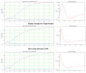
What on the figure below:
1. I used almost the same model (I only add 2-nd lag) from your short motor video and the same control settings.
2. Then i slightly change target position curve - there is trembling on CO curve.
3. Then I apply additional 2-order derivative - CO curve is smooth.
Mathcad file attached.

PID Tuning tool

drbitboy

Lifetime Supporting Member

drbitboy

Lifetime Supporting Member

Peter Nachtwey

Member

destination unknown

Member

MaxK

Member

MaxK

Member

MaxK

Member

Peter Nachtwey

Member

destination unknown

Member

Peter Nachtwey

Member

MaxK

Member

Attachments

MaxK

Member

MaxK

Member

Peter Nachtwey

Member

MaxK

Member

Attachments

Similar Topics